Weaving, one of mankind’s oldest crafts, traces its origins back to Neolithic times (approximately 12,000 years ago). Initially, weaving provided a way to rapidly create objects such as baskets, which were extremely useful in primitive societies. Over time materials and weaving processes were developed to create textiles. This allowed the construction of clothing whose resilience was significantly greater than felt, which is a more primitive pressed fabric.
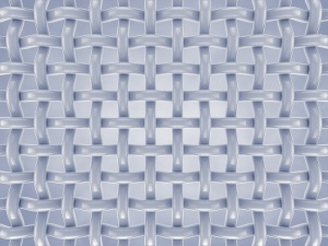
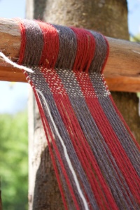
The basic idea in weaving is to interlace threads at right angles. Using a device called a loom, evenly spaced vertical and horizontal threads are woven together. The most basic interlacing involves threads having uniform thickness and color, and consists of alternately passing horizontal threads above and below the vertical threads as shown in the fabric on the right.
Over the centuries, the craft of weaving grew both in scale and complexity. Mechanical devices, called looms, of increasing sophistication and diversity were developed to facilitate a wide variety of weaving processes. By varying thread color, material, and thickness as well as the interleaving pattern, fabrics (including rugs) of incredible beauty were created. Countries/cultures legendary for making beautiful rugs include (but are not limited to): Egypt, Persia, Turkey, Afghan, Chinese, Pakistan, Tibet, and India.


We will use the term weaving algorithm to describe any process that creates a fabric from a set of threads (or yarns). There are many different kinds of weaving algorithms. Some are relatively simple while others are immensely complex.
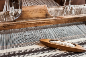
Using this terminology, a loom then is a device (e.g., a machine) used to implement particular kinds of weaving algorithms. When seen from this perspective, a loom can be considered to be a specialized computing device of sorts. There are many different types of looms. Some have mechanics that are quite simple while other looms are intricate machines. Some must be operated by humans while others are operated by motors.
In 1801 the operation of a loom was demonstrated whose capabilities greatly simplified the implementation of complex weaving algorithms such as those used to create brocade, damask, and matelassé patterns. This loom was invented by Joseph Marie Jacquard and became known as the Jacquard Loom or the Jacquard Machine.
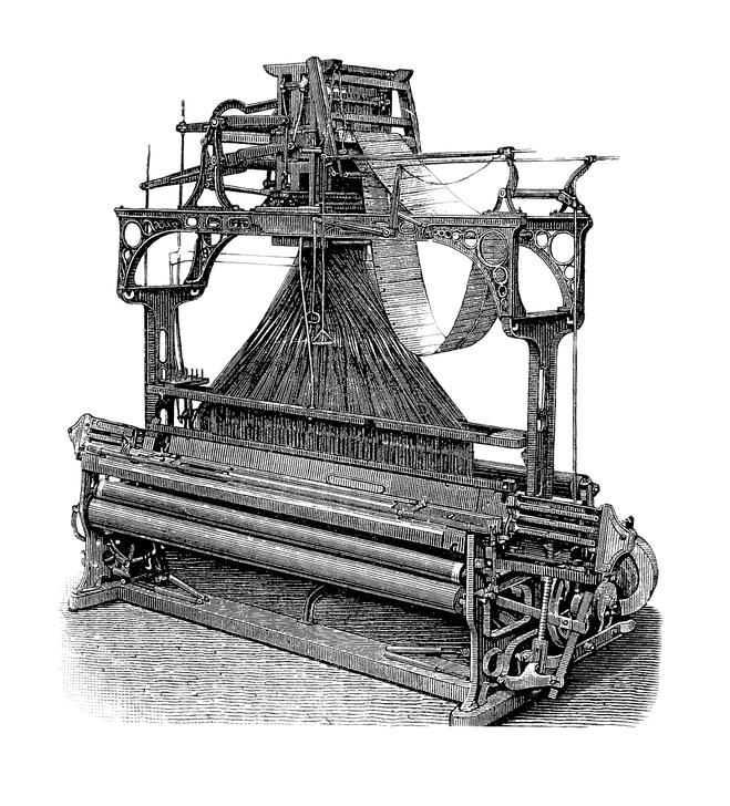
One aspect of the Jacquard Loom that is particularly interesting is that a weaving algorithm is expressed in terms of a sequence of punched cards conceptually similar to those used to store programs that were executed by early computers. In particular, punch cards were commonly used to store computer programs until the early 1980’s.
Rather than being fed into the machine using a card reader, the punched cards of a Jacquard Loom were stitched together into a continuous sequence called a “chain of cards” which, when fed to the machine, controlled its weaving behavior.
Aside: The Babbage Machines
Charles Babbage (1791-1871) is considered to be “the first computer pioneer”. He spent a significant portion of his life developing designs as well as small prototypes for two kinds of computing devices, the difference engine and the analytical engine.
The first kind of device, the difference engine, was a machine that could compute and tabulate polynomial functions through a series of addition operations. The algorithm implemented by Baggage’s difference engines involved calculating finite differences. It this algorithmic feature after which these machines were named.
Conceptually, the behavior of Babbage’s difference engines are similar to complex calculators. The design of the first machine, called Difference Engine No. 1 began in 1821 and ended in 1832 and consisted of around 25,000 parts. The design of the second machine, Difference Engine No. 2, took place during 1847-1849.
Though it contains fewer parts (around 8000), Difference Engine No. 2 essentially has the same computing power as its predecessor. However, the output capabilities of Difference Engine No. 2 are significantly more advanced than Difference Engine No. 1. Among other things, the user (e.g., programmer) could control the size of margins, line height, and insertion of blank lines. It is worth noting that the output capabilities employed by Difference Engine No. 2 were originally developed for the Analytical Engine.
The second kind of device, called an analytical engine, was conceived in 1834 and is similar in many respects to the computing machines of the 20th century. For example, the analytical engine had a memory (called a Store) and processor (called a Mill) and was programmable through punched cards (an idea that originated in the Jacquard Machine). The machine also supported a variety of computing primitives such as conditional branching and iteration.
Lady Ada Lovelace saw Babbage’s analytical engine as being more than just a processor of numbers. She viewed the computational capabilities of the machine in more general terms as a symbol-manipulating device. This idea she conveyed in the following (often quoted) analogy: “We may say most aptly that the Analytical Engine weaves algebraic patterns just as the Jacquard-loom weaves flowers and leaves.”
Regrettably, none of Charles Babbage’s machines where constructed in their entirety in his lifetime. However, some small working portions were constructed. Notably a prototype consisting of 2,000 part that still functions to this very day.
In London in 2002, Charles Babbage’s Difference Engine No. 2 was built in its entirety. The machine consists of 8,000 parts and weighs 5 tons and is shown below. Visit the Computer History Museum for more information about Charles Babbage and his machines as well as a stunning video showing the functioning of the complete Difference Engine No. 2.
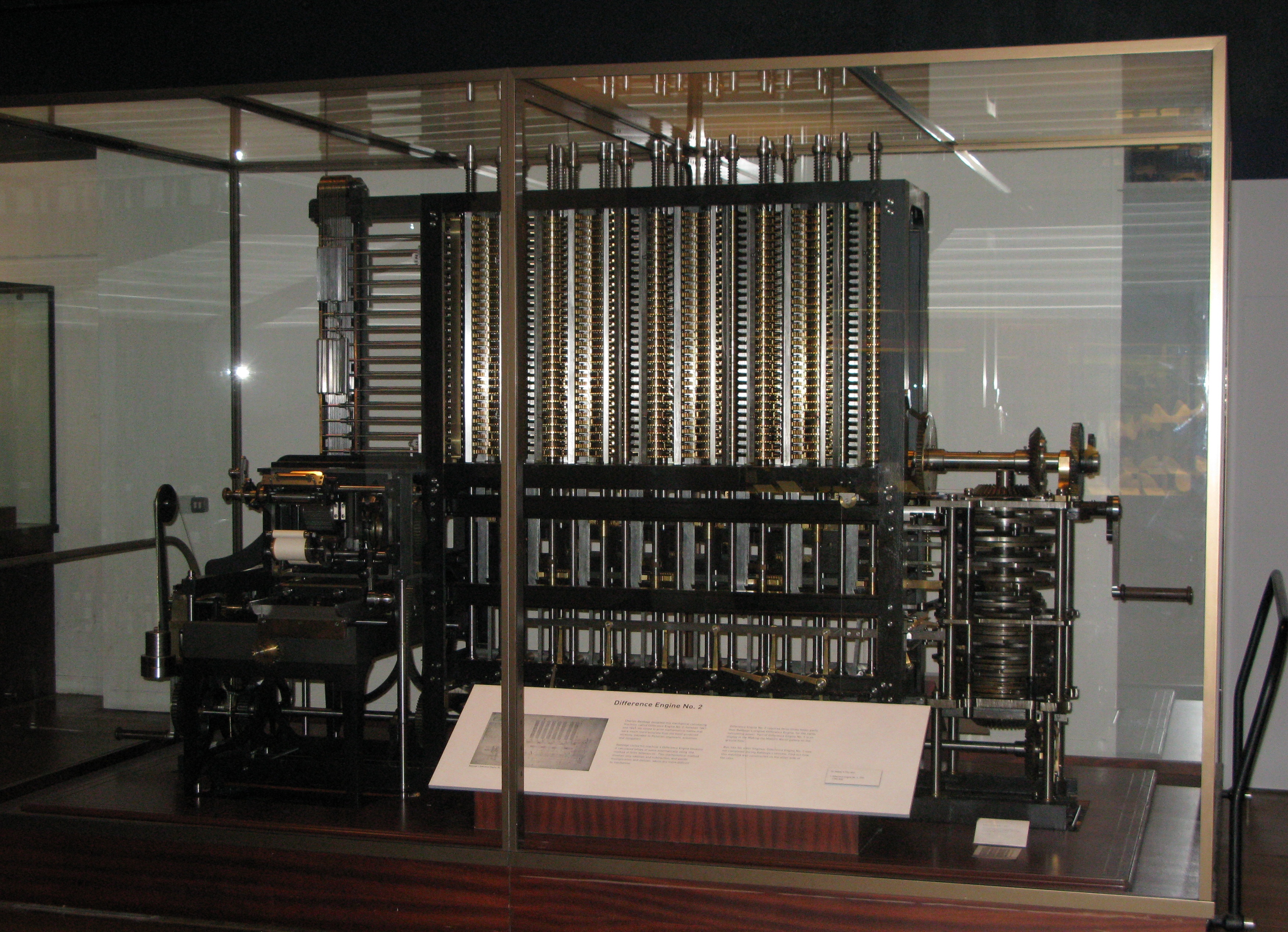
“Babbage Difference Engine” by User:geni – Photo by User:geni. Licensed under GFDL via Wikimedia Commons.
Bricklayer
In Bricklayer, weaving-like algorithms can be implemented through alternating sequences of lines (or rings). Recall that the default overwriting behavior in Bricklayer is that the last brick placed in a cell occupies that cell. Therefore, if two lines cross, the point where they cross will be occupied by a brick belonging to the line which was drawn second (i.e., last). This overwriting behavior can be used to simulate weaving-like behaviors.
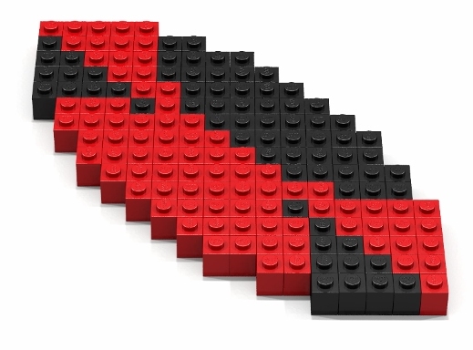
The program shown below draws a sequence of blue and yellow lines. Note that blue and yellow lines are at right angles to one another and are created in an alternating fashion (first blue, then yellow). As a result of this alternation, a pattern emerges where the lines intersect. We use the term weaving pattern when referring to such emerging patterns, and we use the term weaving algorithm to refer to algorithms capable of creating weaving patterns. We say a Bricklayer program implements a weaving algorithm, if the LEGO artifact it produces primarily consists of (or contains) one or more weaving patterns.
open Level_3;

build2D(16,16);
lineXZ (0,0) (15,0) BLUE;
lineXZ (0,0) (0,15) YELLOW;
lineXZ (0,1) (15,1) BLUE;
lineXZ (1,0) (1,15) YELLOW;
lineXZ (0,2) (15,2) BLUE;
lineXZ (2,0) (2,15) YELLOW;
lineXZ (0,3) (15,3) BLUE;
lineXZ (3,0) (3,15) YELLOW;
lineXZ (0,4) (15,4) BLUE;
lineXZ (4,0) (4,15) YELLOW;
lineXZ (0,5) (15,5) BLUE;
lineXZ (5,0) (5,15) YELLOW;

show2D "Basic Weave";
Weaving Patterns
In the context of Bricklayer-based weaving, we use the term Bricklayer fabric (or fabric for short) to describe LEGO artifacts created through weaving algorithms. In Bricklayer, it is possible to create fabrics using a variety of weaving patterns. This special project explores a specific set of weaving algorithms (in other special projects we will explore different kinds of weaving algorithms).
To help us think about and describe (i.e., specify) Bricklayer fabrics created in this special project, we will invent some notation. The notation we present is not fully general, but it will help us abstractly describe certain fabrics created through (alternating) sequences of line segments (and rings). To describe these fabrics we need to develop abstractions for (1) line segments and rings, (2) how line segments and rings change over the course of a sequence, and (3) the length of the sequence (e.g., the number of lines/rings in the sequence).
Line-based Fabrics
We begin by specifying a line segment in terms of (1) the name of the line segment, (2) the start and end points of the line segment, and (3) a brick type. The general form of such a specification is shown below.
Line (segment) names can have numbers associated with them (e.g., line1, line2). This allows us to distinguish one line from another. Below is a concrete example in which two lines, one horizontal and one vertical, are specified.
| Line Segment Name | Line Segment Specifics | |
| line1 | = | (0,0) (15,0) BLUE |
| line2 | = | (0,0) (0,15) YELLOW |
Next, we need to develop some notation that allows us to describe how a sequence of adjacent line segments relate to each other. An example of such sequence is shown below.
(  (0,0) (15,0) BLUE;
   (0,1) (15,1) BLUE;
   (0,2) (15,2) BLUE;
   (0,3) (15,3) BLUE;
   (0,4) (15,4) BLUE;
     (0,5) (15,5) BLUE  )
Note that the above sequence consists of six horizontal lines in which the z components of each line differs from the previous line by +1. Also note that the first line in the sequence corresponds to the definition of line1. We will use the following condensed notation to describe the above sequence.
0
In the condensed form shown above, the line1z+1 denotes the base-pattern used in the specification of our fabric (i.e., our sequence of lines). The subscript z+1 indicates that instances of line1 in the sequence are created by adding 1 to the z components of the points in the definition of line1. The superscript 6 indicates that sequence consists of six lines, and the subscript 0 indicates that the first line in the sequence is line1 itself (i.e., z+0).
| Condensed Form | Expanded Form | |
| ( line1z+1 )6 0 |
= | (
  (0,0) (15,0) BLUE;
  (0,1) (15,1) BLUE;
  (0,2) (15,2) BLUE;
  (0,3) (15,3) BLUE;
  (0,4) (15,4) BLUE;
  (0,5) (15,5) BLUE
) |
Note that the fabric specified in this example involves a base-pattern consisting of a single line and is therefore rather uninteresting. More interesting fabrics can be specified using multi-line base-patterns, multi-ring base-patterns, or even base-patterns that involve both rings and lines.
In this special project, we use the term base-pattern to denote any sequence of subscripted line segments and/or rings which are to be repeated in order to form a fabric. A Bricklayer fabric specification then has the following structure.
initialOffset
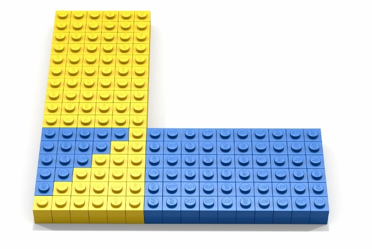
Example 1 – A base-pattern involving two lines.
Consider the condensed and expanded forms of the following fabric specification.
| Condensed Form | Expanded Form | |
| ( line1z+1; line2x+1 )6 0 |
= | (
  (0,0) (15,0) BLUE; (0,0) (0,15) YELLOW;
  (0,1) (15,1) BLUE; (1,0) (1,15) YELLOW;
  (0,2) (15,2) BLUE; (2,0) (2,15) YELLOW;
  (0,3) (15,3) BLUE; (3,0) (3,15) YELLOW;
  (0,4) (15,4) BLUE; (4,0) (4,15) YELLOW;
  (0,5) (15,5) BLUE; (5,0) (5,15) YELLOW
) |
This example shows how a two line base-pattern can be used in the specification of a fabric. Note that the base-pattern involves line1z+1 and line2x+1 and instances of these lines are repeated 6 times (yielding a fabric consisting of 12 individual lines). Also note that line1z+1 indicates that the six instances of line1 are to be generated by adding +1 to the z component of the previous instance of line1, while line2x+1 indicates that the six instances of line2 are to be generated by adding +1 to the x component of the previous instance of line2.
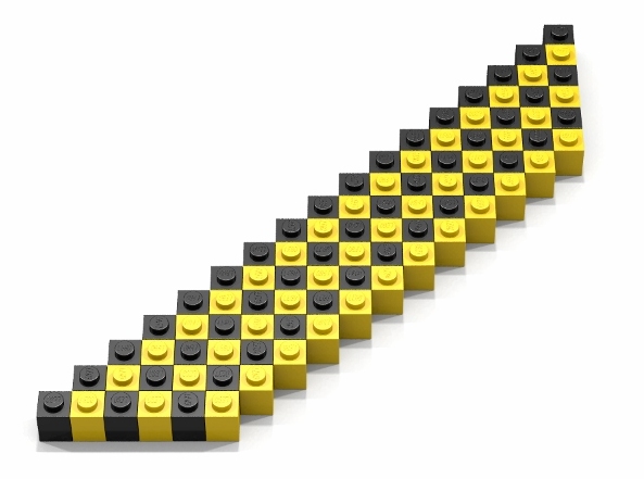
Example 2 – A base-pattern involving diagonal lines.
So far, the examples we have considered involve vertical and horizontal line segments. However, patterns can also contain line segments having other slopes (e.g., diagonal lines). Regardless of the slope, the basic idea is that line sequences in Bricklayer fabrics can be created by “shifting” lines to the left/right or up/down. The property that must be maintained is that related line segments (instances of lines in a sequence) should always have the same slope.
With the exception of horizontal line sequences, all line sequences can be described by (exclusively) specifying changes to the x components of a line. Note that Bricklayer will clip lines that fall outside of the virtual space. Thus, no changes to the z component need be considered. However, horizontal line sequences must be described by specifying changes to the z components of a line.
In this example a fabric is specified using the following two diagonal lines.
| Line Segment Name | Line Segment Specifics | |
| line3 | = | (0,0) (16,16) BLACK |
| line4 | = | (1,0) (17,16) YELLOW |
In the fabric specification below, both lines in the base-pattern have an increment of x+2. This leads to a fabric consisting of an alternating sequence of black and yellow diagonal lines.
| Condensed Form | Expanded Form | |
| ( line3x+2; line4x+2 )3 0 |
= | (
  (0,0) (16,16) BLACK; (1,0) (17,16) YELLOW;
  (2,0) (18,16) BLACK; (3,0) (19,16) YELLOW;
  (4,0) (20,16) BLACK; (5,0) (21,16) YELLOW
) |
A direct translation of the above fabric to a Bricklayer program follows. Note that, in the Bricklayer implementation, the virtual space is 17×17, and that calls to the Bricklayer function lineXZinvolve points lying outside the virtual space. Bricklayer will simply clip (i.e., ignore) portions of lines (i.e., points) that fall outside the virtual space. Therefore, no adjustments need be made to the z components of line segments, and everything behaves as expected.
open Level_3;

build2D(17,17);

lineXZ (0,0) (16,16) BLACK;
lineXZ (1,0) (17,16) YELLOW;

lineXZ (2,0) (18,16) BLACK;
lineXZ (3,0) (19,16) YELLOW;

lineXZ (4,0) (20,16) BLACK;
lineXZ (5,0) (21,16) YELLOW;

show2D "Diagonal Weave";
Ring-based Fabrics
In Bricklayer, fabrics can be constructed using base-patterns containing rings. We specify a ring in terms of its name, radius, brick type and center. The general form of such a specification is shown below.
As was the case with lines, ring names can have numbers associated with them (e.g., ring1, ring2). This allows us to distinguish one ring from another. Below is a concrete example in which two rings are specified.
| Ring Name | Ring Specifics | |
| ring1 | = | 15 BLACK (0,0) |
| ring2 | = | 15 RED (15,15) |
A ring sequence can be constructed from the definition of a ring by increasing/decreasing the radius r of the ring. Note that constructing a sequence of rings in this manner by incrementally changing its radius is conceptually similar to constructing line sequences by incrementally changing either the x components or z components of the points of the line.
Example 3 – A base-pattern involving rings.
In this example we consider a Bricklayer fabric whose specification is shown below.
0
This specification contains a base-pattern consisting of two rings which are used to construct an alternating sequence of black and red rings having smaller and smaller radiuses. The resulting fabric, whose expanded form is shown below, consists of 2*5 = 10 rings.
| Condensed Form | Expanded Form | |
| ( ring1r-1; ring2r-1 )5 0 |
= | (
  15 BLACK (0,0); 15 RED (15,15);
  14 BLACK (0,0); 14 RED (15,15);
  13 BLACK (0,0); 13 RED (15,15);
  12 BLACK (0,0); 12 RED (15,15);
  11 BLACK (0,0); 11 RED (15,15)
) |
The following Bricklayer program creates the ring-based fabric specified in this example.
open Level_3;

build2D(16,16);

ringXZ 15 1 BLACK (0,0);
ringXZ 15 1 RED   (15,15);

ringXZ 14 1 BLACK (0,0);
ringXZ 14 1 RED   (15,15);

ringXZ 13 1 BLACK (0,0);
ringXZ 13 1 RED   (15,15);

ringXZ 12 1 BLACK (0,0);
ringXZ 12 1 RED   (15,15);

ringXZ 11 1 BLACK (0,0);
ringXZ 11 1 RED   (15,15);

show2D "Circular Weave";